workshop01G1:Codefarm
Recursion
import rhinoscriptsyntax as rs
import math
import random
import Rhino as rh
crvList=[]
srfList=[]
ptList=[]
vecList=[]
def G1SKIN(srfa,limit1,limit2,lengthfactor,control,arealimit):
   ptsrf=rs.SurfacePoints(srfa)
   ptsrf.pop(3)
   points=[]
   for pt in ptsrf:
       point=rs.AddPoint(pt)
       points.append(point)
   ptsrf=points
   print ptsrf,'ptsrf'
   pt1= ptsrf [0]
   print pt1,'pt1'
   pt2= ptsrf [1]
   print pt2,'pt2'
   pt3= ptsrf [2]
   print pt3,'pt3'
   crvpts=[]
   crvpts.append(pt1)
   crvpts.append(pt2)
   crvpts.append(pt3)
   crvpts.append(pt1)
   crv=rs.AddCurve(crvpts,1)

   crvList.append(crv)

   obj = rs.CurveAreaCentroid(crv)
   #print obj,'obj'
   ptmid =rs.AddPoint(obj[0])
   print ptmid,'ptmid'
   ptmid1=rs.AddPoint(ptmid)
   ptList.append(ptmid1)
   vecNormal = rs.SurfaceNormal(srfa,(rs.SurfaceClosestPoint(srfa,ptmid)))
   vecNormal = rs.VectorUnitize (vecNormal)
   c = limit1
   d =limit2
   a = random.randint(c,d)
   if a>1.5:
       a=1
   else:
       a=1
   print a,'a'

   scale= rs.Distance(pt1,pt2)/5
   e = lengthfactor
   print e,'e'
   l= a*e
   print l,'l'
   vecNormal= rs.VectorScale(vecNormal, l*scale)
   ptmid = rs.MoveObject (ptmid, vecNormal)
   vecList.append(vecNormal)
   #ptsrf = rh.Geometry.Brep.DuplicateVertices(srfa)
   srfT=[]

   srfM = rs.AddSrfPt([ptmid,pt1,pt2])
   srfT.append(srfM)
   print srfM,'srfM'
   srfN = rs.AddSrfPt ([ptmid,pt2,pt3])
   srfT.append(srfN)
   print srfM,'srfN'
   srfO = rs.AddSrfPt ([ptmid,pt1,pt3])
   srfT.append(srfO)
   print srfO,'srfO'
   #srfT.append(srfM,srfN,srfO)
   for i in range (-1,2):
       k = random.randint(-1,2)
       srfArea= rs.SurfaceArea(srfT[i])
       print srfArea[0],'srfarea'
       x =arealimit
       y=control
       if y ==1 and srfArea[0]>x:
           G1SKIN(srfT[i],limit1,limit2,lengthfactor,control,arealimit)
       else:
           srfList.append(srfT[i])
G1SKIN(surfaceA,limit1,limit2,lengthfactor,control,arealimit)
Cellular Automata Experiment
Cellular Automaton (CA) consist of a grid of cells in which each cell has a state such as on or off. Originally discovered in the 1940's, it was until the 70's that it's popularity begon to rise, thanks to Conway's Game of Life. Stephen Wolfram started to study the CA from the 1980's and published the book New Kind of Science in 2002.
In CA, every cell looks at his neighbour to define it's own state. This can be in 1D, 2D or 3D. For example, in Conway's Game of Life each cell has a state which is alive or dead. In 2D, each cell has 8 neigbours. To determine if the cell goes on or off, there are some rules. For example, if 3 or more neighbours are alive, the cell goes dead because of overpopulation. If no cell is alive, it remains dead as well. If 1 or 2 neigbouring cells are alive, it's own state becomes alive as well.
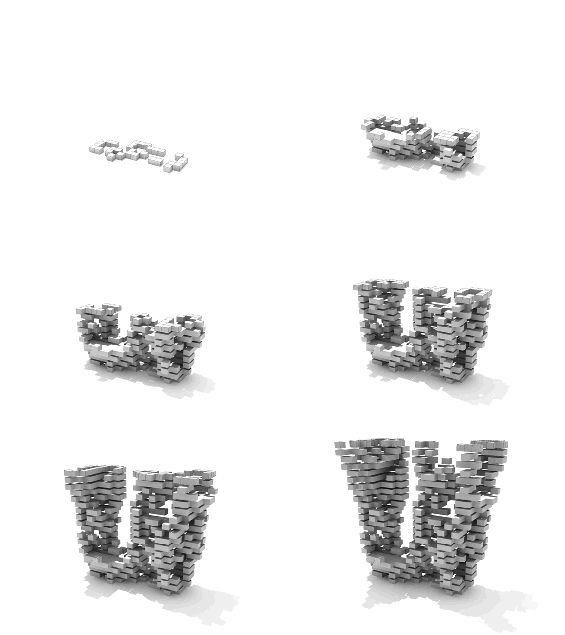
The Gif shows an example to create a 3D structure with boxes.
Source: http://object-e.net/research
L-System Experiments
The L-System, also known as the Lindenmayer System, is created in 1968 by the Hungarian theoretical biologist and botanist A. Lindenmayer. The L-system can be used to describe the behavior of plant cells and to model the growth process of plants.
How does it work:
A plant starts with an axiom and the growth is described by some rules. For example:
Axiom = A, RuleA = A+B-A, RuleB = B-A
Rule A means that every A will be turned in A+B-A; while rule B means that every B will be turned into B-A. Since the Axiom (starting point) is A, This will be turned into A+B-A. In the next iteration every A will be turned into A+B-A again, while the B will be turned into B-A. So for the second iteration we get:
A (Axiom)
A+B-A (1st iteration)
A+B-A+B-A-A+B-A (2nd iteration)
and so on
The '+' and '-' sign tells in which direction the plant grows. For example, when the angle of growth is 60º, the '+' tells to turn 60 degrees in positive direction and the '-' sign tells to turn 60 degrees into the negative direction.
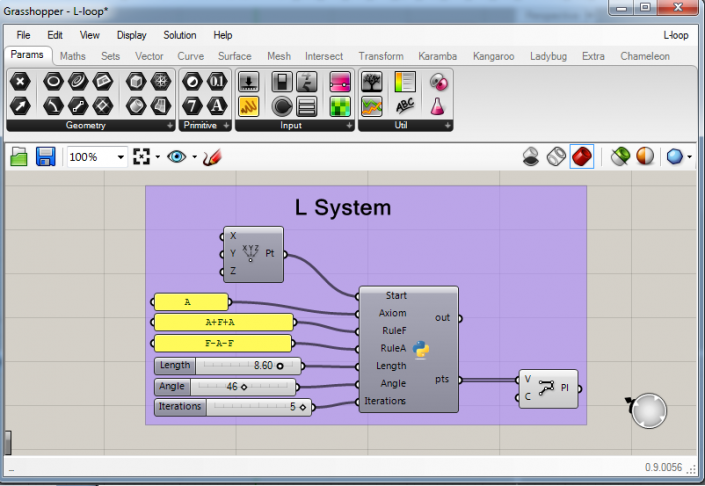
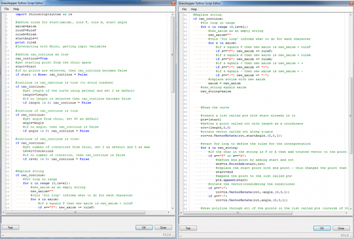
Now, an example written in GH Python for Grasshopper 3D:
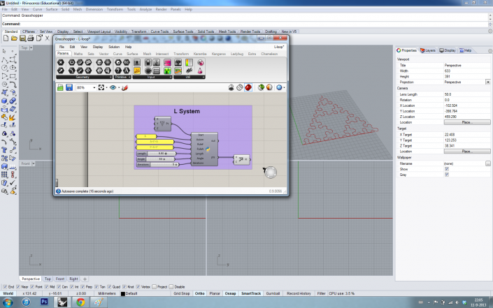
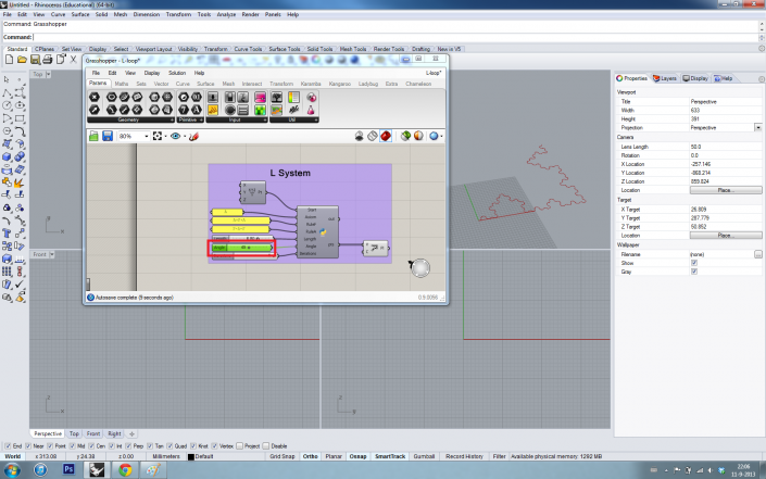
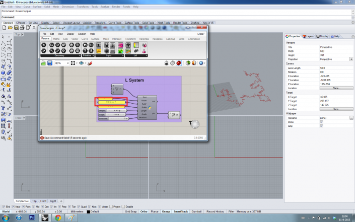
As you can see, in Grasshopper we have a start point, an axiom and two rules which can be changed easily. There are also three sliders for the length, angle and the number of iterations. The outcome is a list of points with a polyline through the points.
test
test
test
